In ClickHouse, brute-force vector search has been supported for several years already. More recently, we added methods for approximate nearest neighbour (ANN) search, including HNSW – the current standard for fast vector retrieval. We also revisited quantisation and built a new data type: QBit. (View Highlight)
Each vector search method has its own parameters that decide trade-offs for recall, accuracy, and performance. Normally, these have to be chosen up-front. If you get them wrong, a lot of time and resources are wasted, and changing direction later becomes painful (View Highlight)
Let’s start with the basics. Vector search is used to find the most similar document (text, image, song, and so on) in a dataset. First, all items are converted into high-dimensional vectors (arrays of floats) using embedding models. These embeddings capture the meaning of the data. By comparing distances between vectors, we can see how close two items are in meaning. (View Highlight)
Approximate Nearest Neighbours (ANN) #
Exact vector search is powerful but slow, and therefore costly. Many applications can tolerate a bit of flexibility. For example, it’s fine if, after listening to Eminem, you’re recommended Snoop Dogg or Tupac. But something has gone very wrong if the next suggestion is this.
That’s why Approximate Nearest Neighbour (ANN) techniques exist. They provide faster and cheaper retrievals at the expense of perfect accuracy. The two most common approaches are quantisation and HNSW.
We’ll look briefly at both, and then see how QBit fits into this picture. (View Highlight)
Suppose our stored vectors are of type Float64, and we’re not happy with the performance. The natural question is: what if we downcast the data to a smaller type?
Smaller numbers mean smaller data, and smaller data means faster distance calculations. ClickHouse’s vectorized query execution engine can fit more values into processor registers per operation, increasing throughput directly. On top of that, reading fewer bytes from disk reduces I/O load. This idea is known as quantisation. (View Highlight)
When quantising, we have to decide how to store the data. We can either:
Keep the quantised copy alongside the original column, or
Replace the original values entirely (by downcasting on insertion).
The first option doubles storage, but it’s safe as we can always fall back to full precision. The second option saves space and I/O, but it’s a one-way door. If later we realise the quantisation was too aggressive and results are inaccurate, there’s no way back. (View Highlight)
There are many data structures designed to find the nearest neighbour without scanning all candidates. We call them indexes. Among them, HNSW is often seen as the monarch.
(View Highlight)
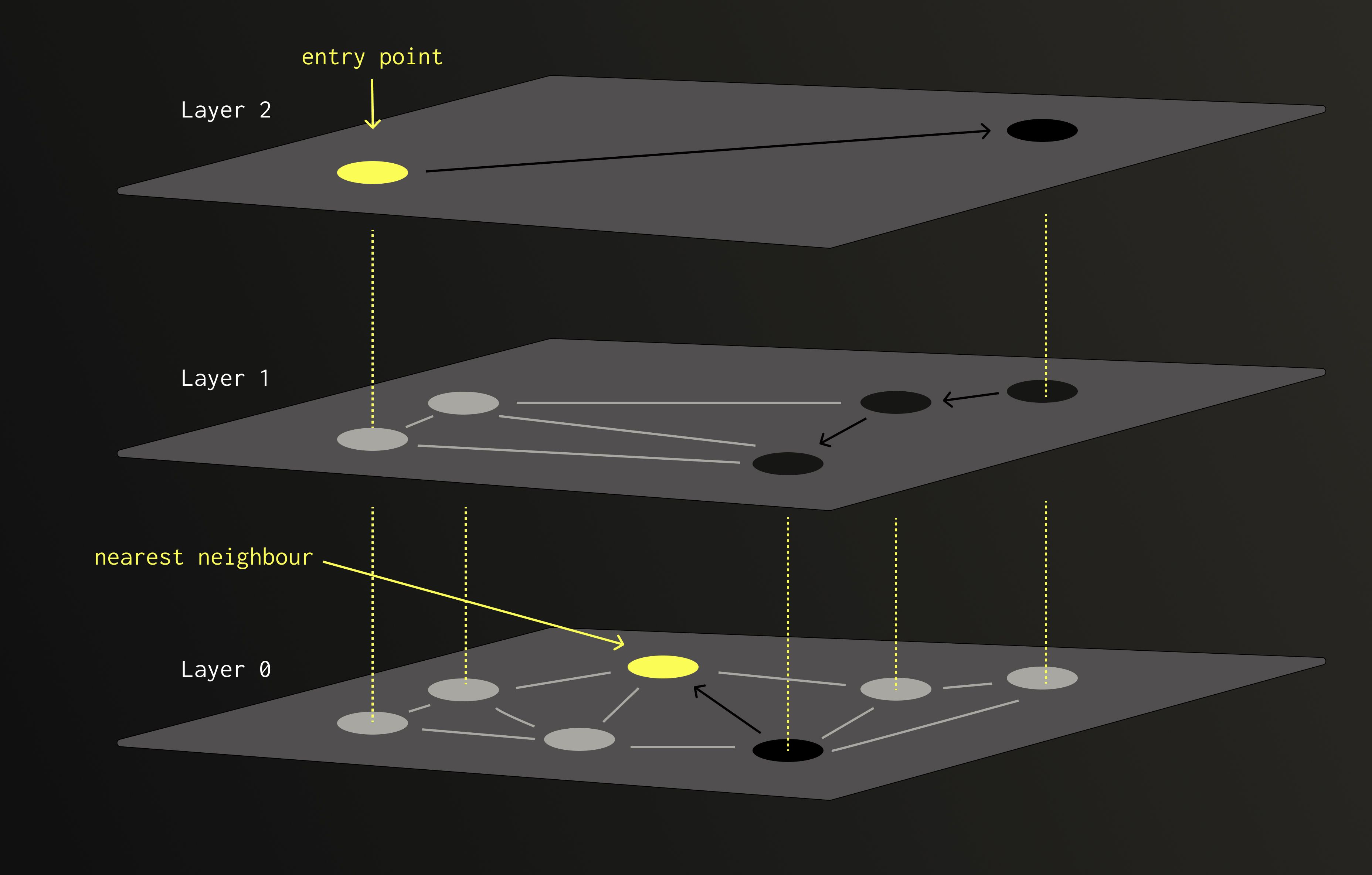
HNSW is built from multiple layers of nodes (vectors). Each node is randomly assigned to one or more layers, with the chance of appearing in higher layers decreasing exponentially.
When performing a search, we start from a node at the top layer and move greedily towards the closest neighbours. Once no closer node can be found, we descend to the next, denser layer, and continue the process. The higher layers provide long-range connections to avoid getting trapped in local minima, while the lower layers ensure precision.
Because of this layered design, HNSW achieves logarithmic search complexity with respect to the number of nodes. Far faster than the linear scans used in brute-force search or quantisation-based methods. (View Highlight)
The main bottleneck is memory. ClickHouse uses the usearch implementation of HNSW, which is an in-memory data structure that doesn’t support splitting. As a result, larger datasets require proportionally more RAM. Quantising the data before building the index can help reduce this footprint, but many HNSW parameters still have to be chosen in advance, including the quantisation level itself. And this is exactly the rigidity that QBit set out to address. (View Highlight)
This approach solves the main limitation of traditional quantisation. There’s no need to store duplicated data or risk making values meaningless. It also avoids the RAM bottlenecks of HNSW, since QBit works directly with the stored data rather than maintaining an in-memory index.
Most importantly, no upfront decisions are required. Precision and performance can be adjusted dynamically at query time, allowing users to explore the balance between accuracy and speed with minimal friction.
Although QBit speeds up vector search, its computational complexity remains O(n). In other words: if your dataset is small enough for an HNSW index to fit comfortably in RAM, that is still the fastest choice. (View Highlight)
When data is inserted into a QBit column, it is transposed so that all first bits line up together, all second bits line up together, and so on. We call these groups.
Each group is stored in a separate FixedString(N) column: fixed-length strings of N bytes stored consecutively in memory with no separators between them. All such groups are then bundled together into a single Tuple, which forms the underlying structure of QBit. (View Highlight)
If we start with a vector of 8×Float64 elements, each group will contain 8 bits. Because a Float64 has 64 bits, we end up with 64 groups (one for each bit). Therefore, the internal layout of QBit(Float64, 8) looks like a Tuple of 64×FixedString(1) columns.
If the original vector length doesn’t divide evenly by 8, the structure is padded with invisible elements to make it align to 8. This ensures compatibility with FixedString, which operates strictly on full bytes. For example, in the picture above, the vector contains 5 Float64 values. It would be padded by three zeroes producing 8×Float64, which is then transposed into a Tuple of 64×FixedString(1). Or, if we started with 76×BFloat16 elements, we would pad it to 80×BFloat16 and transpose it into a Tuple of 16×FixedString(10). (View Highlight)
Before we can calculate distances, the required data must be read from disk and then untransposed (converted back from the grouped bit representation into full vectors). Because QBit stores values bit-transposed by precision level, ClickHouse can read only the top bit planes needed to reconstruct numbers up to the desired precision.
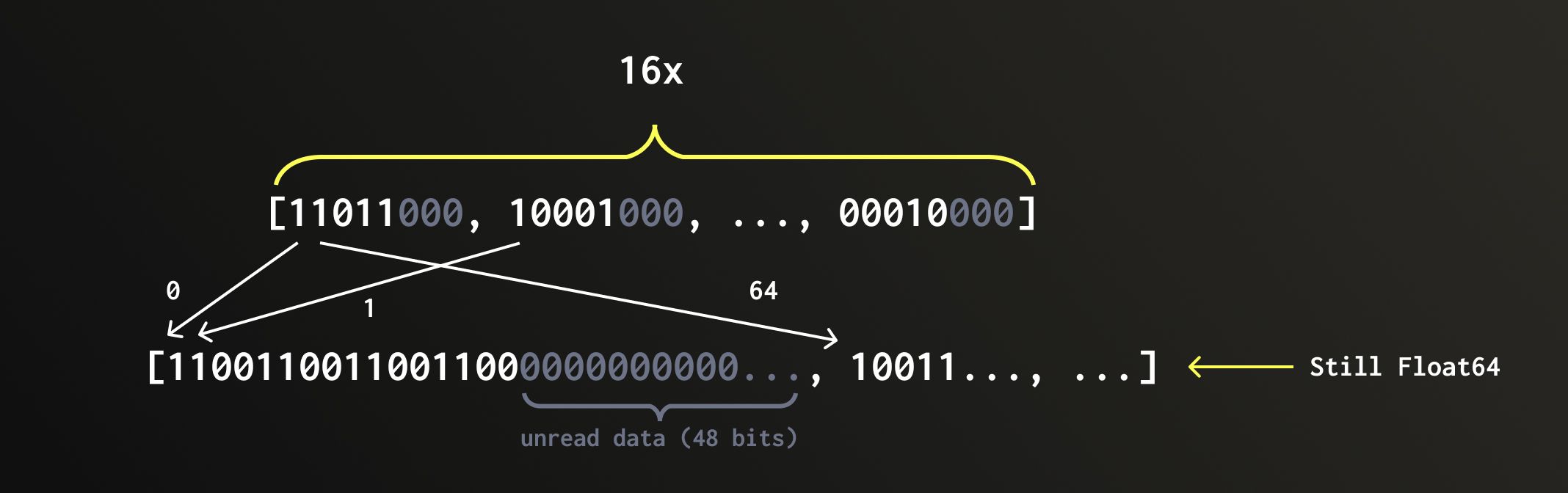
In the query above, we use a precision level of 16. Since a Float64 has 64 bits, we only read the first 16 bit planes, skipping 75% of the data.
After reading, we reconstruct only the top portion of each number from the loaded bit planes, leaving the unread bits zeroed out.
(View Highlight)
Calculation optimisation #
One might ask whether casting to a smaller type, such as Float32 or BFloat16, could eliminate this unused portion. It does work, but explicit casts are expensive when applied to every row. Instead, we can downcast only the reference vector and treat the QBit data as if it contained narrower values (“forgetting” the existence of some columns), since its layout often corresponds to a truncated version of those types. But not always! (View Highlight)
Let’s start with the simple case where the original data is Float32, and the chosen precision is 16 bits or fewer. BFloat16 is a Float32 truncated by half. It keeps the same sign bit and 8-bit exponent, but only the upper 7 bits of the 23-bit mantissa. Because of this, reading the first 16 bit planes from a QBit column effectively reproduces the layout of BFloat16 values. So in this case, we can (and do) safely convert the reference vector (the one all the data in QBit is compared against) to BFloat16 and treat the QBit data as if it were stored that way from the start. (View Highlight)
Float64, however, is a different story. It uses an 11-bit exponent and a 52-bit mantissa, meaning it’s not simply a Float32 with twice the bits. Its structure and exponent bias are completely different. Downcasting a Float64 to a smaller format like Float32 requires an actual IEEE-754 conversion, where each value is rounded to the nearest representable Float32. This rounding step is computationally expensive and cannot be replaced with simple bit slicing or permutation.
The same holds when the precision is 16 or smaller. Converting from Float64 to BFloat16 is effectively the same as first converting to Float32 and then truncating that to BFloat16. So here too, bit-level tricks won’t help. (View Highlight)
The main performance difference between regular quantised columns and QBit columns is the need to untranspose the bit-grouped data back into vector form during search. Doing this efficiently is critical. ClickHouse has a vectorized query execution engine, so it makes sense to use it to our advantage. You can read more about vectorisation in this ClickHouse blog post.
In short, vectorisation allows the CPU to process multiple values in a single instruction using SIMD (Single-Instruction-Multiple-Data) registers. The term originates from the fact that SIMD instructions operate on small batches (vectors) of data. Individual elements within these vectors are of fixed length and are typically referred to as lanes. (View Highlight)
There are two common approaches to vectorising algorithms:
Auto-vectorisation. Write an algorithm in such a way that the compiler will figure out the concrete SIMD instructions itself. As compilers can only do this with very simple straight-forward functions, usually such a way is only achievable if the architecture of your system is carefully designed around an auto-vectorising algorithm, like here.
Intrinsics. Write the algorithm using explicit intrinsics: special functions that compilers map directly into CPU instructions. These are platform dependent, but offer full control. (View Highlight)
We loop through all FixedString columns of the QBit (64 of them for Float64). Within each column, we iterate over every byte of the FixedString, and within each byte, over every bit.
If a bit is 0, we apply a zero mask to the destination at the corresponding position. If a bit is 1, we apply a mask that depends on its position within the byte. For example, if we are processing the first bit, the mask is 10000000; for the second bit, it becomes 01000000, and so on. The operation we apply is a logical OR, merging the bit from the source into the destination byte. (View Highlight)
Let’s now look at the second iteration (steps 3 and 4 from above) using AVX-512, an instruction set that’s common across modern CPUs. In this example, we’re unpacking the second FixedString(1) group and each bit here contributes to the secondbit of eight resulting Float64 values. (View Highlight)
We ran benchmarks on the HackerNews dataset, which contains around 29 million comments represented as Float32 embeddings. We measured the speed of searching for a single new comment (using its embedding) and computed the recall based on 10 new comments.
Recall here is the fraction of true nearest neighbours that appear among the top-k retrieved results (in our case, k = 20). Granularity is how many bit groups we read.
(View Highlight)
We achieved nearly 2× speed-up with a good recall. More importantly, we can now control the speed-accuracy balance directly, adjusting it to match the workload.
Take the Float64 recall results with a grain of salt: these embeddings are simply upcast versions of Float32, so the lower half of the Float64 bits carries little to none information, thus removing them didn’t affect the recall as much as it can. Speed-up values, however, are fully reliable in both cases. (View Highlight)

 (View Highlight)
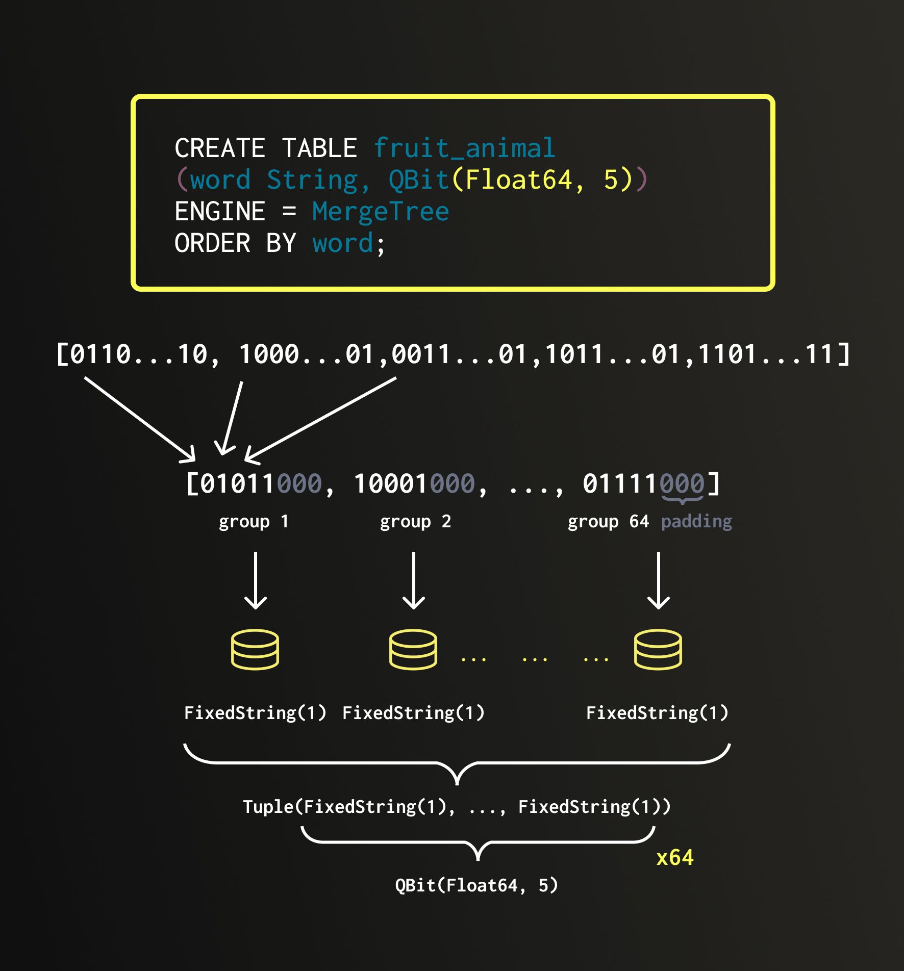 When data is inserted into a QBit column, it is transposed so that all first bits line up together, all second bits line up together, and so on. We call these groups.
Each group is stored in a separate
When data is inserted into a QBit column, it is transposed so that all first bits line up together, all second bits line up together, and so on. We call these groups.
Each group is stored in a separate 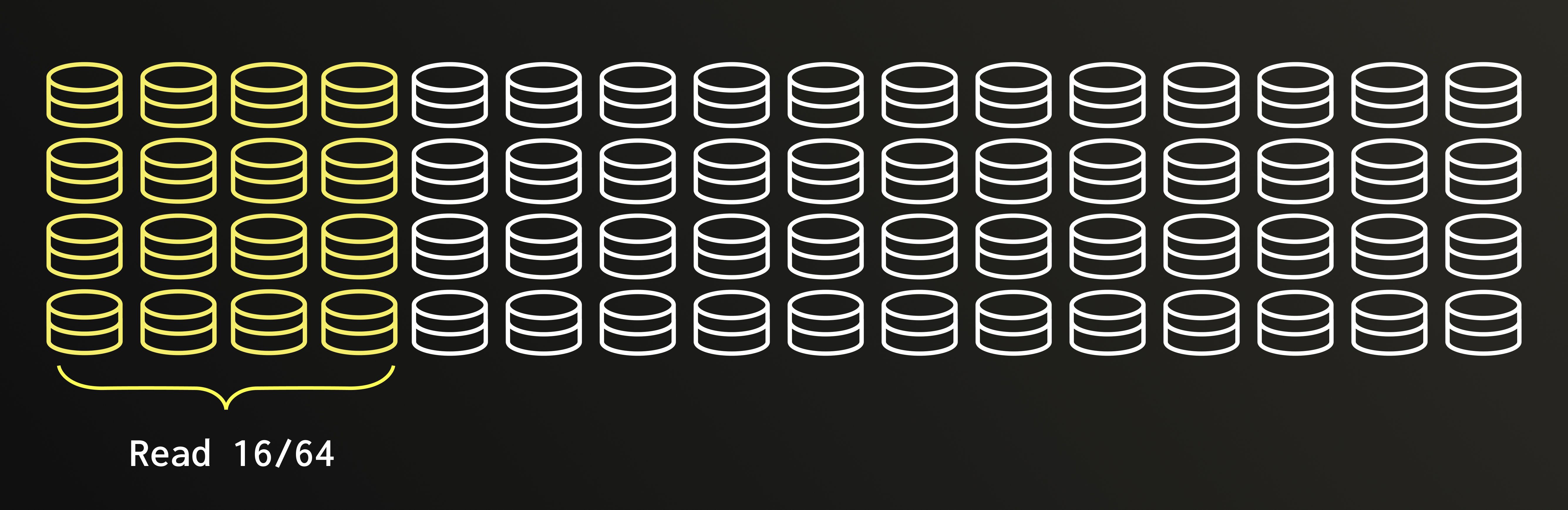 After reading, we reconstruct only the top portion of each number from the loaded bit planes, leaving the unread bits zeroed out.
 (View Highlight)
 Let’s start with the simple case where the original data is
 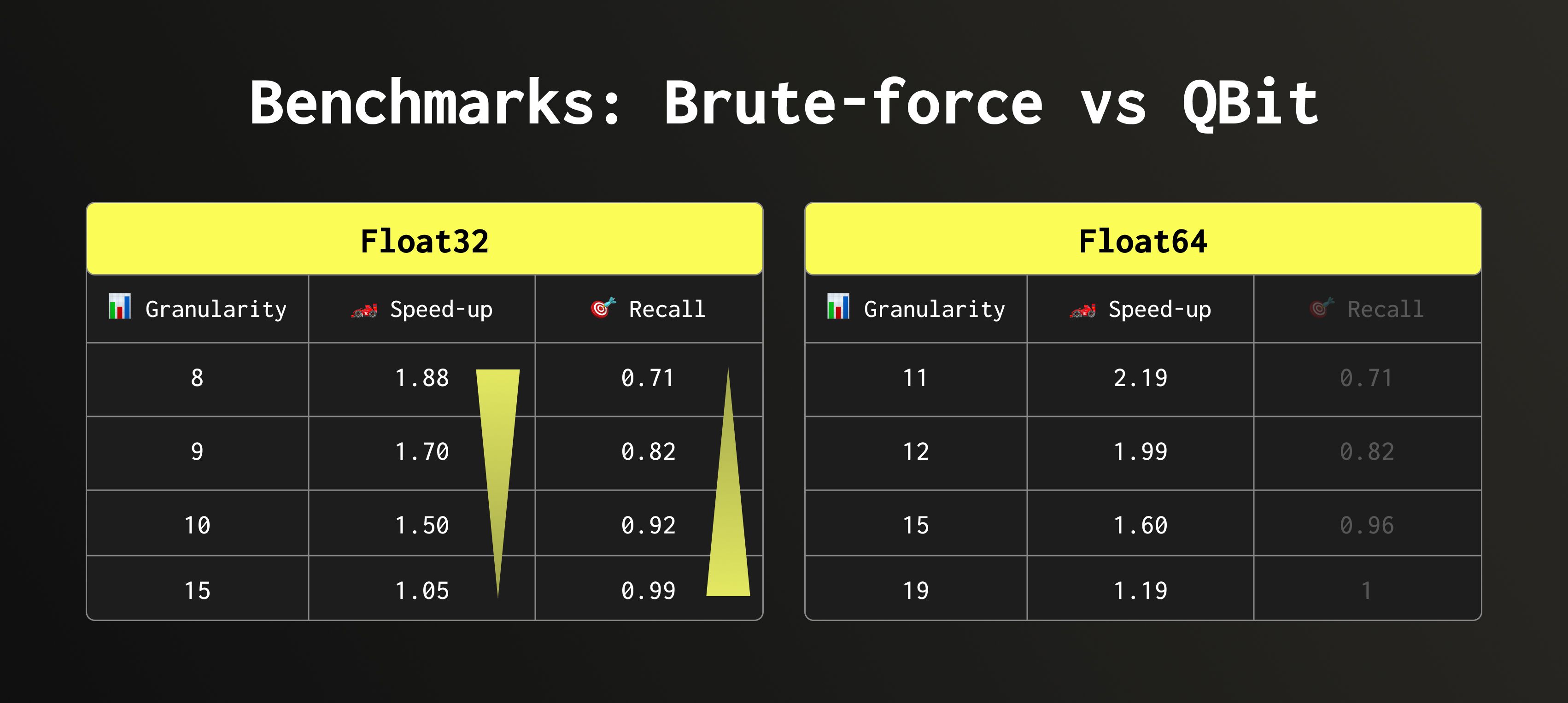 (View Highlight)