Today we release GLiNER2.5, the most significant upgrade to the GLiNER architecture to date. Across a suite of 16 benchmarks spanning diverse classification and extraction tasks, GLiNER2.5 achieves higher overall average F1 scores in comparison to GLiNER2, including a significant 24.75-point gain on XNLI. We release three variants on Hugging Face under Apache 2.0: gliner2.5-base-v1 (0.2B), gliner2.5-multi-v1 (0.3B), and gliner2.5-small-v1 (74M). (View Highlight)
Two changes drive this release. The architecture replaces span enumeration with boundary prediction, scoring entity start and end positions directly, so inference scales linearly with document length. And the training data was generated with the Fastino Data Agent rather than assembled from existing datasets, covering task combinations, document formats, and languages that no public dataset does. (View Highlight)
Together, these bring five new capabilities to GLiNER users: long-context extraction and classification over full documents, unlimited span length for entities of any size, joint entity and relation extraction for coherent knowledge graphs, constrained classification for outputs that are valid by construction, and richer extraction context with span attributes. (View Highlight)
Long-Context Extraction for Full Documents
GLiNER2.5 handles long documents in two ways, one in the model and one in the library.
First, the model itself takes longer inputs. Removing explicit span representations cut memory use enough to train on sequences up to 4,096 words, so most contracts, reports, and transcripts fit in a single forward pass without chunking.
Second, the library now offers native chunking. Every extraction task has a long-document variant with batch versions: entities, classification, JSON schemas, relations, and generic extraction. The document is split into overlapping word chunks, extraction runs on each, and every span is remapped to character offsets in the original document. Duplicates across overlaps are merged under deterministic policies you control, and any returned span can be checked directly against the source text.
GLiNER2 required you to truncate, or write your own chunking and handle offset remapping and cross-chunk duplicates yourself. Now extracting obligations from a full contract or tracking entities across an hour-long transcript is one call, and the schema API is the same at any length. (View Highlight)
Unlimited Span Length for Whole-Entity Extraction
GLiNER2.5 removes the maximum span width that constrained GLiNER2. An entity can now begin at the first token and end at the last, so spans of any length are extractable: full postal addresses, clause-length legal references, complete product titles, multi-line table cells.
GLiNER2 enumerated candidate spans up to a fixed width, typically around twelve words, and anything longer was structurally invisible. The model did not score it poorly; it never scored it at all. Users worked around this by raising the width limit, which increased compute with every step, or by extracting fragments and stitching them together afterwards.
Image showing unlimited span length for whole-entity extraction, a new feature of GLiNER2.5
The boundary prediction architecture removes the limit rather than raising it. Because the model scores where an entity starts and where it ends instead of scoring enumerated spans, there is no width axis in the computation at all. A forty-word indemnification clause costs the same to locate as a two-word name, and no configuration is required.
This changes what is practical to extract. Legal and contract work can treat whole clauses as entities. Document processing can capture full addresses and references as single spans rather than reassembled parts. And because span length no longer trades against compute, schemas can include long entity types without a performance penalty. (View Highlight)
Joint Information Extraction for Coherent Knowledge Graphs
GLiNER2.5 extracts entities and relations together as a single, globally decoded graph, which means that every relation in the output connects entities that actually exist in the result, and the structure as a whole obeys the rules of your schema.
When entities and relations are scored independently, the combined output is frequently inconsistent. Relations may reference entities that fell below the extraction threshold, a person may be assigned two employers where the schema intends one, and hierarchical relations may contain cycles instead of forming a valid tree. Resolving these inconsistencies has traditionally been left to the user, requiring post-hoc filtering rules.
With GLiNER2.5, the user declares entity types, typed relations, and structural rules in a joint schema and the returned output is guaranteed to conform. This is what makes the output suitable for knowledge graphs specifically. A knowledge graph is only as reliable as its least consistent edge, and when triples are extracted independently, every ingestion pipeline needs logic to reject dangling references, enforce cardinality, and break cycles. Joint decoding moves that work into the extraction itself, so what reaches the graph is already well-formed.
from gliner2.joint_ie import JointIE, JointIEConfig
joint = JointIE.from_pretrained(“fastino/gliner2.5-multi-v1”)
schema = (
joint.create_schema()
.entities([“person”, “organization”, “location”])
.relation(“works_for”, “person”, “organization”, unique_head=True)
.relation(“located_in”, “organization”, “location”, unique_head=True)
.no_self_loops()
)
text = “Tim Cook leads Apple in Cupertino. Sundar Pichai runs Google in Mountain View.”
result = joint.extract(text, schema, config=JointIEConfig(optimizer=“beam”, beam_size=32))
for rel in result.relations:
head = result.entity(rel.head)
tail = result.entity(rel.tail)
print(f” {head.text} -{rel.type}-> {tail.text} (conf {rel.confidence:.2f})“)
Apple -located_in-> Cupertino (conf 0.96)
Google -located_in-> Mountain View (conf 0.95)
Tim Cook -works_for-> Apple (conf 0.87)
Sundar Pichai -works_for-> Google (conf 0.87)
The model achieves this by scoring all candidate entities and relations in a single forward pass. A beam search then assembles the highest-scoring combination, checking each candidate against the declared rules as the solution is built rather than filtering the output afterwards. Because invalid combinations are never admitted into the search, the returned graph satisfies the schema by construction.
image showing joint information extraction for coherent knowledge graphs in GLiNER2.5
This is a substantial departure from GLiNER2, where relation extraction returned independently thresholded triples and consistency was the user’s responsibility. With GLiNER2.5, the model’s output can be treated as a well-formed graph from the moment it is returned, which makes it possible to populate knowledge graphs, build entity-linking pipelines, and feed downstream systems directly, without a validation layer in between. (View Highlight)
Constrained Classification
With GLiNER2, classification joined extraction as a first-class capability, spanning multi-label, multi-class, hierarchical, and multi-task setups. GLiNER2.5 builds on this foundation by enforcing user-declared constraints during decoding, which guarantees valid outputs and allows predictions on one task to inform another.
from gliner2 import AutoExtractor
model = AutoExtractor.from_pretrained(“fastino/gliner2.5-multi-v1”)
model.classify_text(
“Delete the temporary file”,
{“intent”: {“labels”: [“read”, “write”, “delete”]}},
)
schema = (
ClassificationSchema()
.single(“intent”, [“read”, “write”, “delete”])
.multi(
“effects”,
[“read_only”, “create”, “modify”, “delete”],
min_labels=1,
max_labels=2,
)
.constrain(
C.implies((“intent”, “delete”), (“effects”, “delete”)),
C.implies((“intent”, “read”), (“effects”, “read_only”)),
C.excludes((“intent”, “read”), (“effects”, “delete”)),
C.excludes((“intent”, “read”), (“effects”, “modify”)),
)
)
result = clf.classify(“Delete the temporary file from /tmp”, schema)
print(result.value(“intent”)) # “delete”
print(result.selected(“effects”)) # (“delete”,)
print(result.feasible) # True
print(result.to_dict())
Traditional unconstrained classification can result in predictions that contradict each other across tasks. Consider GLiGuard, our guardrail model, which classifies both the overall safety of a prompt and the type of harm present when it is unsafe. Without constraints, these two tasks are decoded independently, so a prompt can be labeled safe while simultaneously being flagged for prompt injection, a contradiction that downstream code then has to detect and resolve. With constrained classification, a single declared rule, that a harm type may only be assigned when the prompt is labeled unsafe, makes this contradiction impossible: the decoder never admits the invalid combination in the first place. And if no valid assignment exists at all, the classifier raises an error rather than returning an invalid classification. (View Highlight)
Richer Extraction Context with Span Attributes
Span attributes allow the model to apply descriptive labels to the spans it extracts, such as a mention of a product and whether that mention is positive or negative in sentiment. GLiNER2.5 decodes these attributes in the same forward pass as the entities themselves, so entities come back qualified rather than flat and lacking context.
schema = (
model.create_schema()
.entities([“product”])
.entity_attributes({
“sentiment”: AttributeGroup(
[“positive”, “negative”, “neutral”],
applies_to=[“product”],
qualify_labels=True,
)
})
)
result = model.extract(
text,
schema,
include_spans=True,
include_confidence=True,
)
print(result)
When creating the extraction schema, the user defines attribute groups, each a small set of possible values, and attaches them to entity types, so that a group can apply to all entities or only to specific ones. A group can assign a single value per span or several, with a confidence threshold the user controls. Because the attributes are part of the schema, the model scores them alongside the entities in one pass, and each returned span carries its attribute values directly.
GLiNER2 could classify and extract in the same pass, but its classifications applied to the input as a whole rather than to each span, so entities came back flat. With GLiNER2.5, the attributes are decoded span-by-span within the original forward pass, so a single call returns the spans and their qualifications together. (View Highlight)
The GLiNER2.5 Boundary Architecture
GLiNER2.5 is built on a new architecture that changes how the model locates entities in text. Earlier GLiNER models enumerated candidate spans: every possible start position paired with every allowed width, each scored against the schema’s entity types. This design tied computation to a width axis and imposed a hard ceiling on how long an extracted entity could be.
The new architecture removes the span enumeration entirely. The shared encoder still processes the text and the schema’s queries together in one pass, but instead of scoring spans, the model predicts where entities begin and end: for each query, it produces start and end scores over the text’s token boundaries and inside scores over the tokens themselves. An entity is located by its boundaries rather than matched against an enumerated list of candidates, and no full position-by-position score matrix is ever built.
From these scores, a sparse proposal stage selects the most promising start and end boundaries per query and pairs them, with no restriction on how far apart a start and end may sit, so a span can open at the first token and close at the last. A reranking head then scores each proposed candidate using the boundary evidence and the span’s content, and relation candidates are drawn from this same pool rather than through a separate extraction path. Computation stays linear in sequence length for a fixed schema and candidate budget, and the maximum entity width that constrained earlier GLiNER models is gone. (View Highlight)
Use cases
GLiNER2.5’s capabilities are most visible in what they let you build. Each of the use cases below previously required code around the model, chunking logic, validation layers, second passes, or handing the task to an LLM; each now runs as a single call against a single small model.
• Model and agent routing. Route tasks to sub-agents, tools, or model tiers with the routing decision and task type decoded jointly under your compatibility rules, rather than as independent predictions that downstream code must reconcile.
• Agent guardrails. Screen agent actions with a classifier whose safety verdict and harm type are decoded under a declared rule, so a contradictory verdict is no longer possible.
• Knowledge graph construction for agent memory. Give agents a queryable graph of people, projects, and commitments, built from the documents, email, and chat history they read, where joint decoding keeps every edge typed and the structure consistent as the graph grows.
• PII detection and redaction. Find personal data across an entire contract or transcript rather than its first window, with each span carrying a global character offset for redaction at the source.
• Contract review. Extract parties, obligations, and termination clauses from all three hundred pages, not the portion that fits in the model window, and verify each span against the source text.
• Clinical extraction. Pull symptoms and medications with negation status and dosage form attached to each span in the same forward pass, instead of re-classifying every extracted span in a second one. (View Highlight)
Conclusion
GLiNER2.5 rests on a new boundary prediction architecture that scores where entities begin and end rather than enumerating candidate spans, and this foundation is what makes its five new capabilities possible: long-context extraction over entire documents, unlimited span length extraction, joint entity and relation extraction, constrained classification, and extraction of span attributes. Together they open use cases that previously required either a pipeline of models or a large language model: populating knowledge graphs directly from raw text, extracting structured records from full contracts and reports, and running guardrail or triage classifiers whose outputs are valid by construction. Across our benchmark suite, GLiNER2.5 matches or exceeds GLiNER2’s overall macro-average F1 scores, reaching up to 56.17 F1, demonstrating that the new architecture does not trade away the extraction quality the GLiNER family is known for. (View Highlight)

 (View Highlight)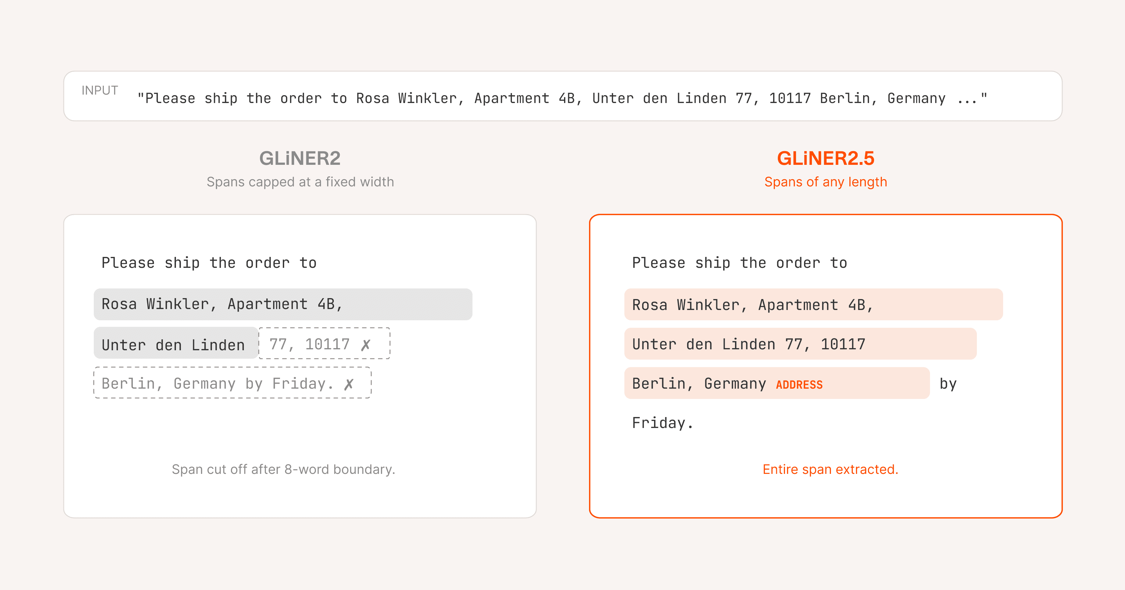

 (View Highlight)