Metadata
- Author: Piotr Migdał
- Full Title: Don’t Use Cosine Similarity Carelessly
- URL: https://p.migdal.pl/blog/2025/01/dont-use-cosine-similarity?utm_campaign=Data_Elixir&utm_source=Data_Elixir_519
Highlights
- Let’s look at three sentences: • A: “Python can make you rich.” • B: “Python can make you itch.” • C: “Mastering Python can fill your pockets.” If you treated them as raw IDs, there are different strings, with no notion of similarity. Using string similarity (Levenshtein distance), A and B differ by 2 characters, while A and C are 21 characters apart. Yet semantically (unless you’re allergic to money), A is closer to C than B. (View Highlight)
- These vectors are quite long - text-embedding-3-large has up 3072 dimensions - to the point that we can truncate them at a minimal loss of quality. When we calculate cosine similarity, we get 0.750 between A and C (the semantically similar sentences), and 0.576 between A and B (the lexically similar ones). These numbers align with what we’d expect - the meaning matters more than spelling! (View Highlight)
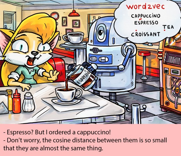
- When comparing vectors, there’s a temptingly simple solution that every data scientist reaches for, often without a second thought — cosine similarity (View Highlight)
- Geometrically speaking, it is the cosine of the angle between two vectors. However, I avoid thinking about it this way - we’re dealing with spaces of dozens, hundreds, or thousands of dimensions. Our geometric intuition fails us in such high-dimensional spaces, and we shouldn’t pretend otherwise. From a numerical perspective, it is a dot product with normalized vectors. It has some appealing properties: • Identical vectors score a perfect 1. • Random vectors hover around 0 (there are many dimensions, so it averages out). • The result is between -1 and 1. Yet, this simplicity is misleading. Just because the values usually fall between 0 and 1 doesn’t mean they represent probabilities or any other meaningful metric. The value 0.6 tells little if we have something really similar, or not so much. And while negative values are possible, they rarely indicate semantic opposites — more often, the opposite of something is gibberish. (View Highlight)
- Pearson correlation can be seen as a sequence of three operations: • Subtracting means to center the data. • Normalizing vectors to unit length. • Computing dot products between them. When we work with vectors that are both centered () and normalized (), Pearson correlation, cosine similarity and dot product are the same. In practical cases, we don’t want to center or normalize vectors during each pairwise comparison - we do it once, and just use dot product. In any case, when you are fine with using cosine similarity, you should be as fine with using Pearson correlation (and vice versa). (View Highlight)
- Using cosine similarity as a training objective for machine learning models is perfectly valid and mathematically sound. As we just seen, it’s a combination of two fundamental operations in deep learning: dot product and normalization. The trouble begins when we venture beyond its comfort zone, specifically when:
• The cost function used in model training isn’t cosine similarity (usually it is the case!).
• The training objective differs from what we actually care about. (View Highlight)
- Tags: favorite
- A common scenario involves training with unnormalized vectors, when we are dealing with a function of dot product - for example, predicting probabilities with a sigmoid function and applying log loss cost function. Other networks operate differently, e.g. they use Euclidean distance, minimized for members of the same class and maximized for members of different classes. The normalization gives us some nice mathematical properties (keeping results between -1 and +1, regardless of dimensions), but it’s ultimately a hack. Sometimes it helps, sometimes it doesn’t — see the aptly titled paper Is Cosine-Similarity of Embeddings Really About Similarity?. (View Highlight)
- We are safe only if the model itself uses cosine similarity or a direct function of it - usually implemented as a dot product of vectors that are kept normalized. Otherwise, we use a quantity we have no control over. It may work in one instance, but not in another. If some things are extremely similar, sure, it is likely that many different measures of similarity will give similar results. But if they are not, we are in trouble. In general, it is a part of a broader subject of unsupervised machine vs self-supervised learning. In the first one, we take an arbitrary function and we get some notions or similarity. Yet, there is no way to evaluate it. The second one, self-supervised learning, is a predictive model, in which we can directly evaluate the quality of prediction. (View Highlight)
- And here is the second issue - even if a model is explicitly trained on cosine similarity, we run into a deeper question: whose definition of similarity are we using? Consider books. For a literary critic, similarity might mean sharing thematic elements. For a librarian, it’s about genre classification. For a reader, it’s about emotions it evokes. For a typesetter, it’s page count and format. Each perspective is valid, yet cosine similarity smashes all these nuanced views into a single number — with confidence and an illusion of objectivity. (View Highlight)
- The best approach is to directly use LLM query to compare two entries. So, first, start with a powerful model of your choice. Then, we can write something in the line of:
“Is {sentence_a} a plausible answer to {sentence_b}?” This way we harness the full power of an LLM to extract meaningful comparisons - powerful enough to find our keys in pockets, and wise enough to understand the difference between questions and answers. We typically want our answers in structured output - what the field calls “tools” or “function calls” (which is really just a fancy way of saying “JSON”). Since many models love Markdown (as they were trained on it), my default template looks like this:
{question} ## A {sentence_a} ## B {sentence_b}However, in most cases this approach is impractical - we don’t want to run such a costly operation for each query. Unless our dataset is very small, it would be prohibitively expensive. Even with a small dataset, the delays would be noticeable compared to a simple numerical operation. (View Highlight) - So, we can go back to using embeddings. But instead of blindly trusting a black box, we can directly optimize for what we actually care about by creating task-specific embeddings. There are two main approaches: • Fine-tuning (teaching an old model new tricks by adjusting its weights). • Transfer learning (using the model’s knowledge to create new, more focused embeddings). (View Highlight)
- Which one we use is ultimately a technical question - depending on the access to the model, costs, etc. Let’s start with a symmetric case. Say we want to ask, “Is A similar to B?” We can write this as: where , and is a matrix that reduces the embedding space to dimensions we actually care about. Think of it as decluttering — we’re keeping only the features relevant to our specific similarity definition. But often, similarity isn’t what we’re really after. Consider the question “Is document B a correct answer to question A?” (note the word “correct”) and the relevant probability: where and . The matrices and transform our embeddings into specialized spaces for queries and keys . It’s like having two different languages and learning to translate between them, rather than assuming they’re the same thing. This approach works beautifully for retrieval augmented generation (RAG) too, as we usually care not only about similar documents but about the relevant ones. But where do we get the training data? We can use the same AI models we’re working with to generate training data. Then feed it into PyTorch, TensorFlow, or your framework of choice. (View Highlight)
- Another approach is to preprocess the text before embedding it. Here’s a generic trick I often use — I ask the model:
“Rewrite the following text in standard English using Markdown. Focus on content, ignore style. Limit to 200 words.” This simple prompt works wonders. It helps avoid false matches based on superficial similarities like formatting quirks, typos, or unnecessary verbosity. Often we want more - e.g. to extract information from a text while ignoring the rest. For example, let’s say we have a chat with a client and want to suggest relevant pages, be it FAQ or product recommendations. A naive way would be to compare their discussion’s embedding with the embeddings of our pages. A better approach is to first transform the conversation into a structured format focused on needs: “You have a conversation with a client. Summarize their needs and pain points in up to 10 Markdown bullet points, up to 20 words each. Consider both explicit needs and those implied by context, tone, and other signals.” Similarly, rewrite each of your pages in the same format before embedding them. This strips away everything that isn’t relevant to matching needs with solutions. This approach has worked wonders in many of my projects. Perhaps it will work for you too. (View Highlight)
- Let’s recap the key points: • Cosine similarity gives us a number between -1 and 1, but don’t mistake it for a probability. • Most models aren’t trained using cosine similarity - then the results are just “some sort of correlations” without any guarantees. • Even when a model is trained with cosine similarity, we need to understand what kind of similarity it learned and if that matches our needs. • To use vector similarity effectively, there are a few approaches: • Train custom embeddings on your specific data • Engineer prompts to focus on relevant aspects • Clean and standardize text before embedding (View Highlight)