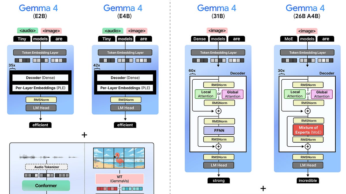
There are four models in the Gemma 4 family:
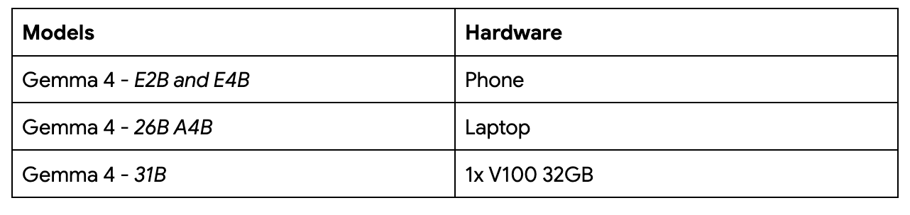
• Gemma 4 - E2B – A dense model with per-layer embeddings, which make them effectively 2 billion parameters
• Gemma 4 - E4B – A dense model with per-layer embeddings, which make them effectively 4 billion parameters
• Gemma 4 - 31B– A dense model with 31 billion parameters
• Gemma 4 - 26B A4B – A Mixture of Experts (MoE) model with 26 billion total parameters of which 4 billion are activated during inference. (View Highlight)
By having a broad range of model sizes, you can choose whichever model best suits your use case and whether it actually fits on your hardware:
(View Highlight)
Aside from a wide range of sizes, all models are multimodal and can reason about input images. They were trained to handle many images of varying sizes (more on that later!).
I’m especially interested in trying out the small models a bit more since they not only support input images and text, but also audio. (View Highlight)
There are a number of things that were changed compared to Gemma 3 that relate to all model sizes:
• Interleaving Layers – Global attention is always the last layer
• K=V – The Keys are set to be equivalent to the Values only for the global attention
• p-RoPE – Low-frequency-pruned RoPE applied to the embeddings (View Highlight)
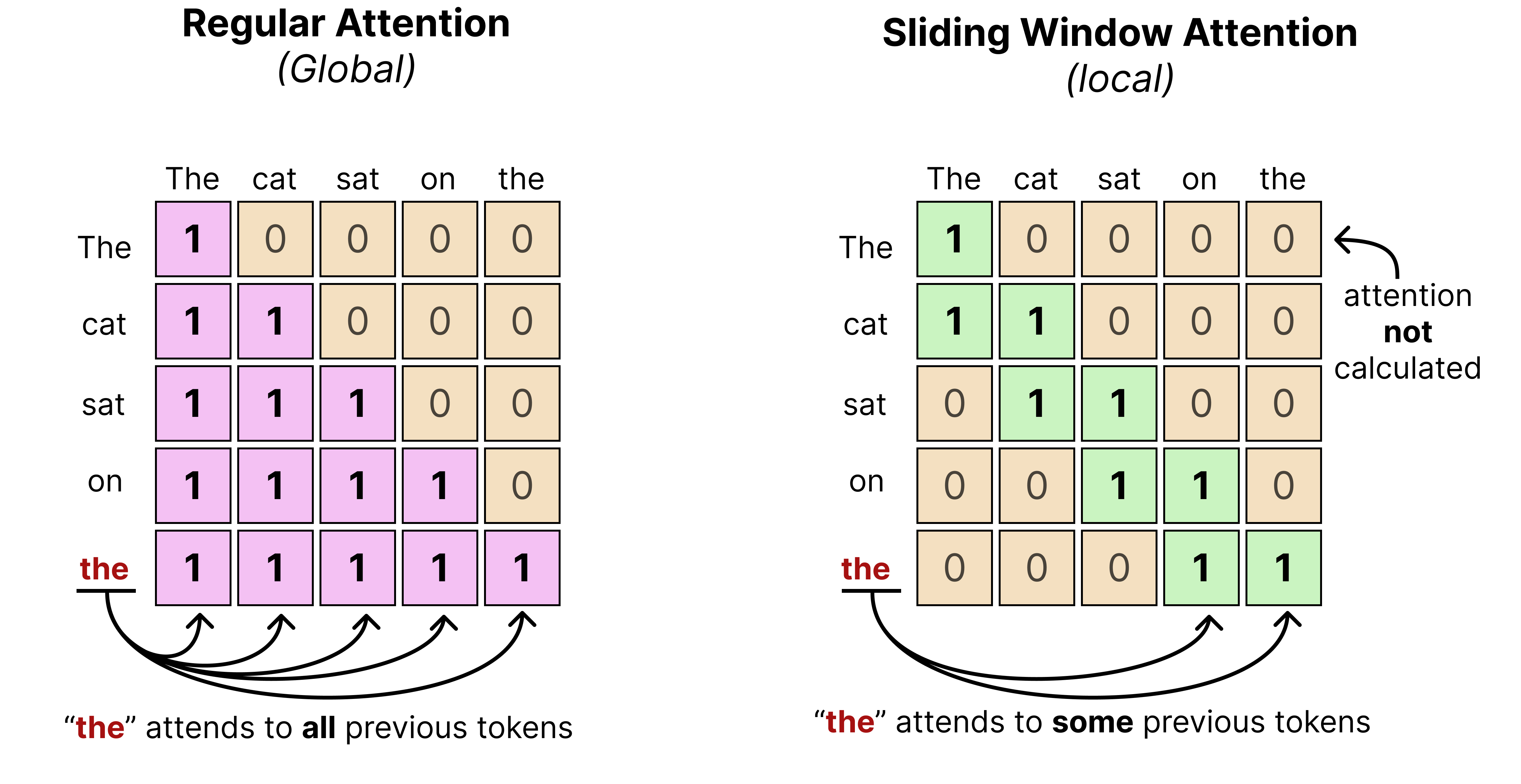
Like Gemma 3, Gemma 4 interleaves layers of local attention (also called “sliding window attention”) with global attention (which is regular or “full” attention).
Remember that in global attention, every token attends to all tokens that came before it. Sliding window attention, however, only attends to tokens within a certain limit. This significantly reduces the compute needed to calculate the full attention.
(View Highlight)
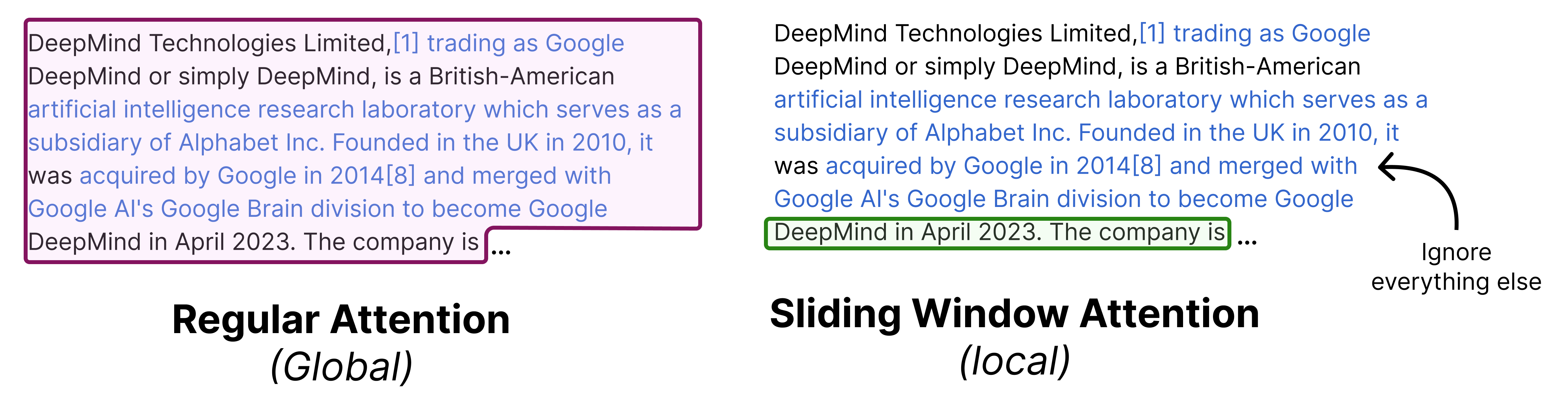
In practice, that means that when text is processed using a sliding window, it may only see a part of the entire sequence rather than the entire thing. The “sliding” then refers to the idea of continuously moving the sequence in view as the number of tokens are being generated.
You typically fix the number of tokens it can see previously. In the case of Gemma 4 models, the smaller models (E2B and E4B) have a sliding window of 512 tokens and the larger models (26B A4B and 31B) have a sliding window of 1024 tokens. (View Highlight)
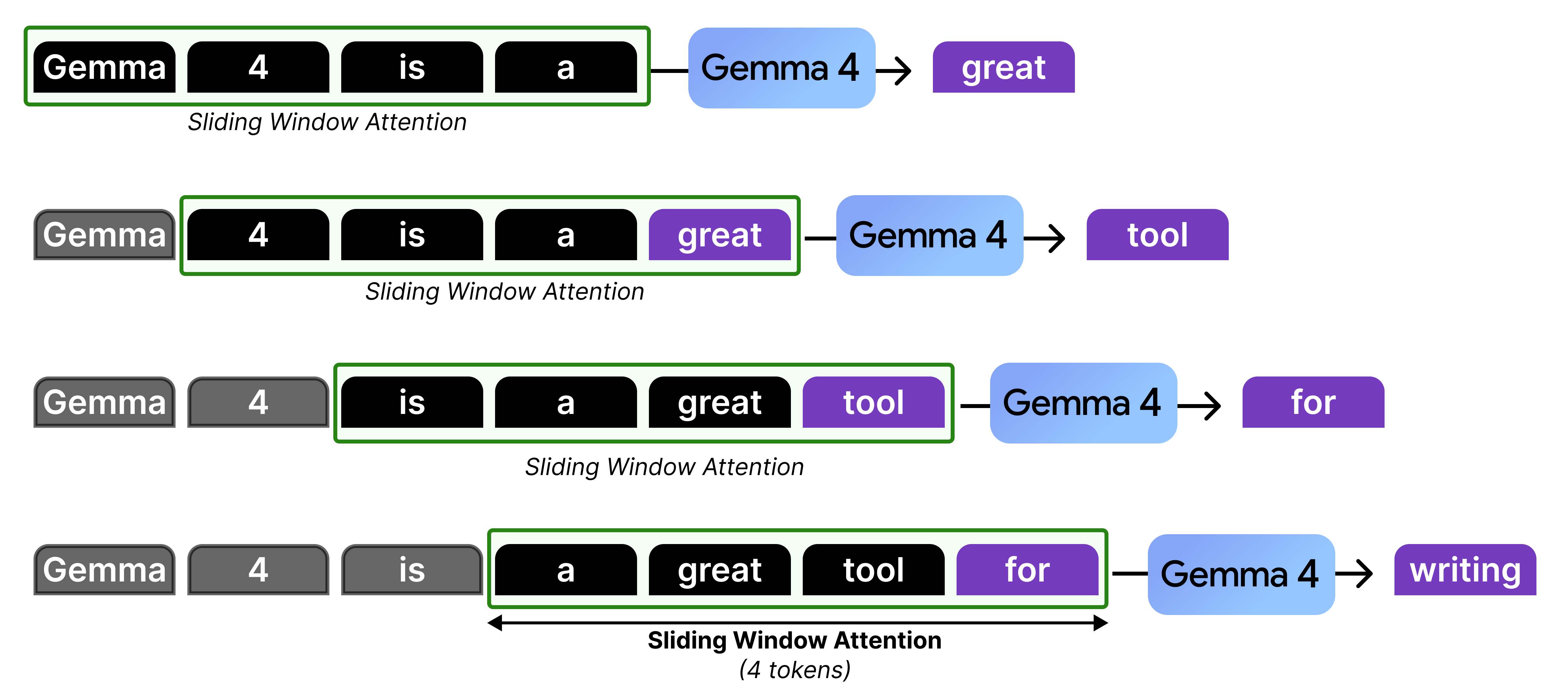
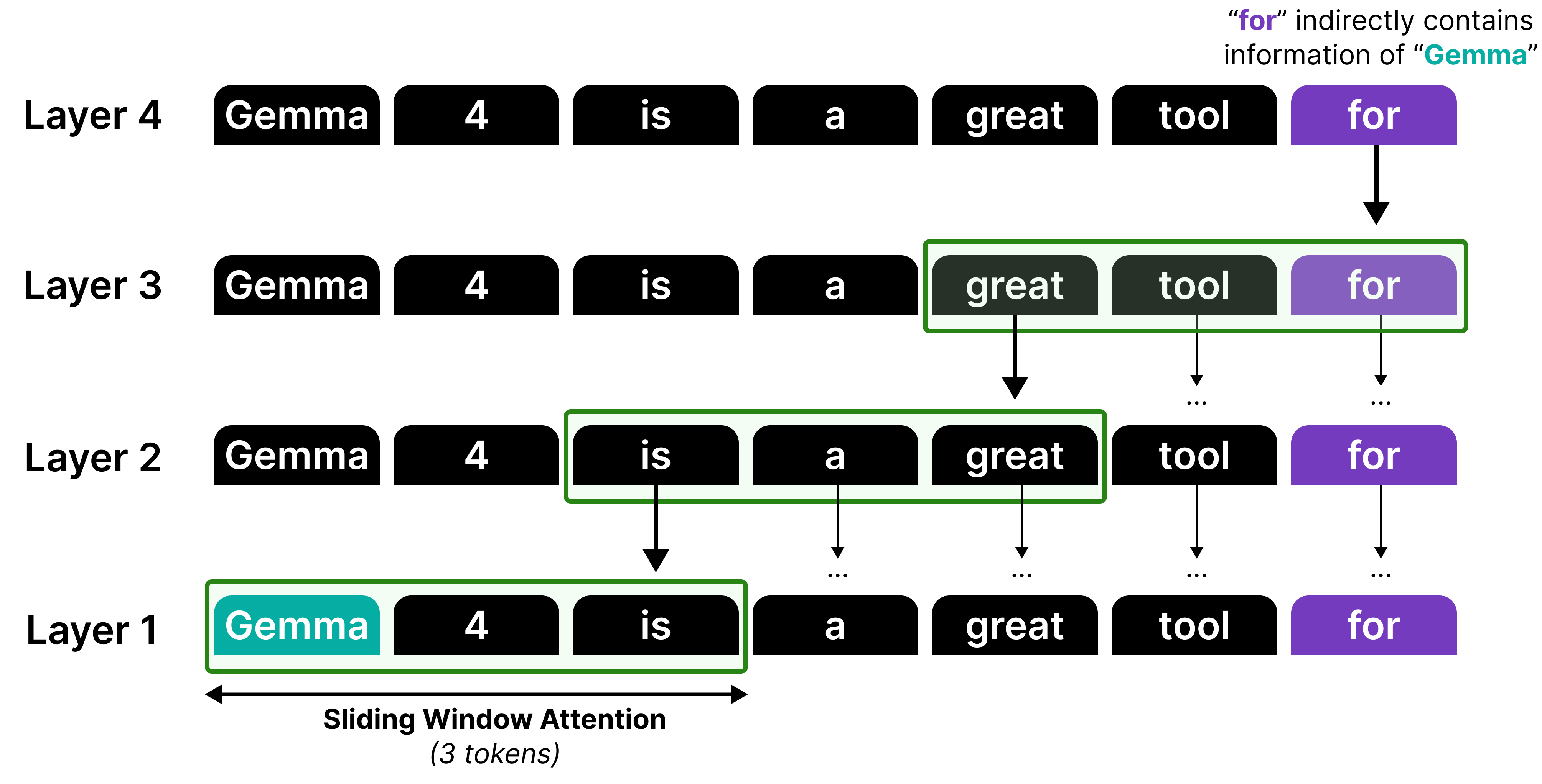
Let’s go through an example with a sliding window of 4 tokens to see what is happening at each token generation:
In our example, there is only attention given to the last four tokens which at some point in the generation starts to “ignore” the ones that came before that. However, it is actually not forgetting the representations that it calculated in the previous steps. The hidden states allow for the attention to be passed along the attention mechanism from previous layers and steps all the way to the current token.
(View Highlight)
Although information can be propagated by stacking sliding windows, it is not a perfect recall or attention mechanism. Think of it like a game of telephone, information gets diluted each time it passes through another layer!
Therefore, much like in Gemma 3, local attention and global attention layers are interleaved such that the model does attend to the full sequence at times to better capture the global structure. (View Highlight)
In Gemma 3, this interleaving was generally in a 4:1 pattern with 4 layers of local attention followed by a single layer of global attention. However, Gemma 3 - 4B for instance had 34 layers, which means its last layer used local attention rather than global attention. This was changed in the Gemma 4 models to make sure that the last layer is always global attention.
(View Highlight)
The 4:1 pattern, however, is only for the E2B as all other variants have a 5:1 pattern where they start with 5 layers of local attention followed by a single layer of global attention. We can visualize this pattern side-by-side to also demonstrate the depth of these models.
(View Highlight)
Making Global Attention more Efficient
Interleaving local attention with global attention is an interesting way of making a Large Language Model more efficient. However, it is not a free lunch. The global attention layers still attend to the entire context, which is a costly and slow process.
In this section, we explore various tricks that Gemma 4 uses to make those global attention layers more efficient! (View Highlight)
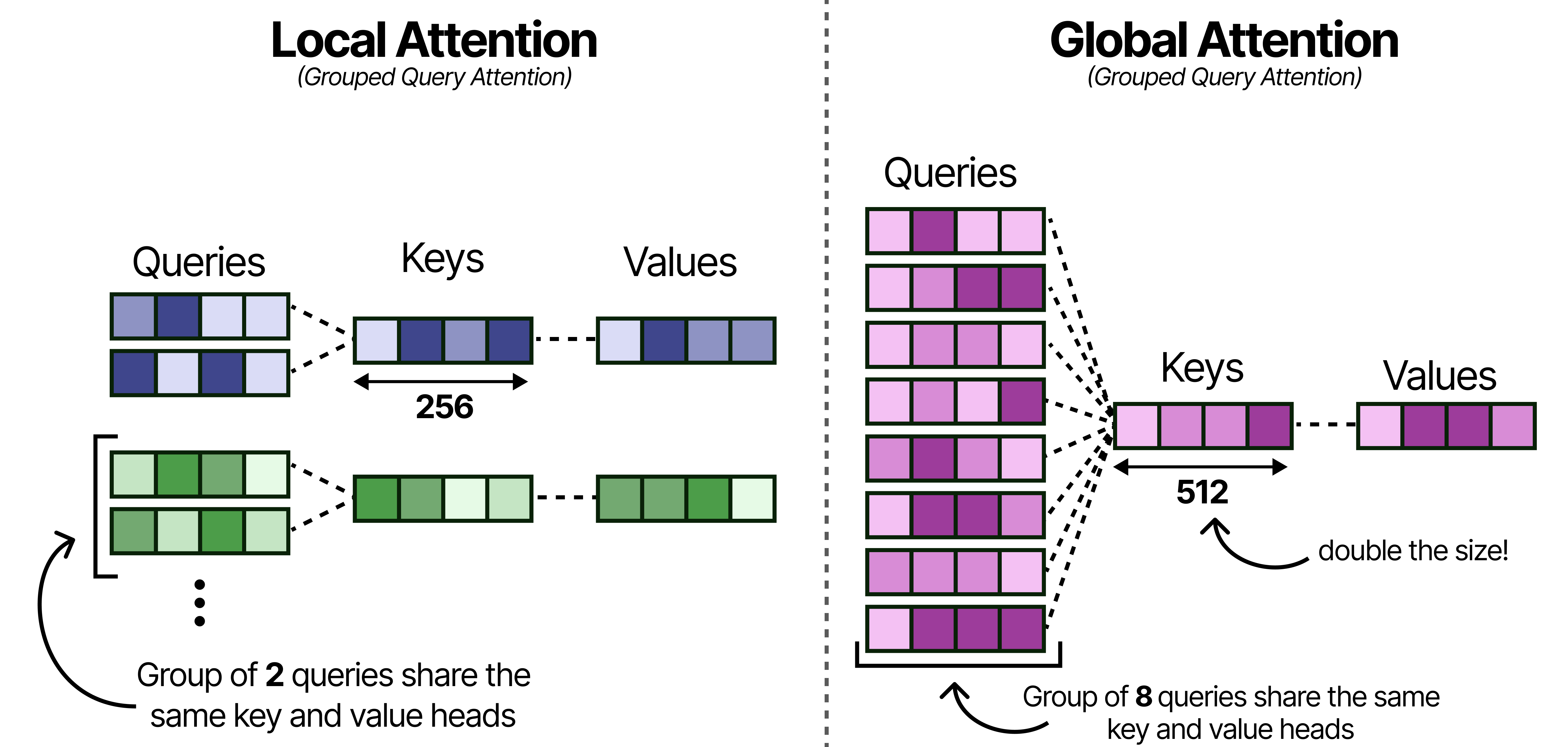
Much like Gemma 3, these models use Grouped Query Attention (GQA) which allows the Query heads to share KV-values which reduces the amount of caching that needs to be done. The local attention layers use GQA and have 2 Query heads sharing one KV head.
With Gemma 4, the global attention layers are made more efficient by having 8 Query heads to share one KV head. This drastically reduces the caching needed of the KV values since global attention by itself already has a lot it needs to store (the entire context) compared to the small context of the local attention layers.
(View Highlight)
Note that reducing the number of keys and values per head may hurt performance and so to compensate for that, the size of the Keys was doubled!
Doubling the dimensions of the Keys does fill up the KV-cache quite a bit, so let’s explore another interesting trick for reducing the KV-cache. (View Highlight)
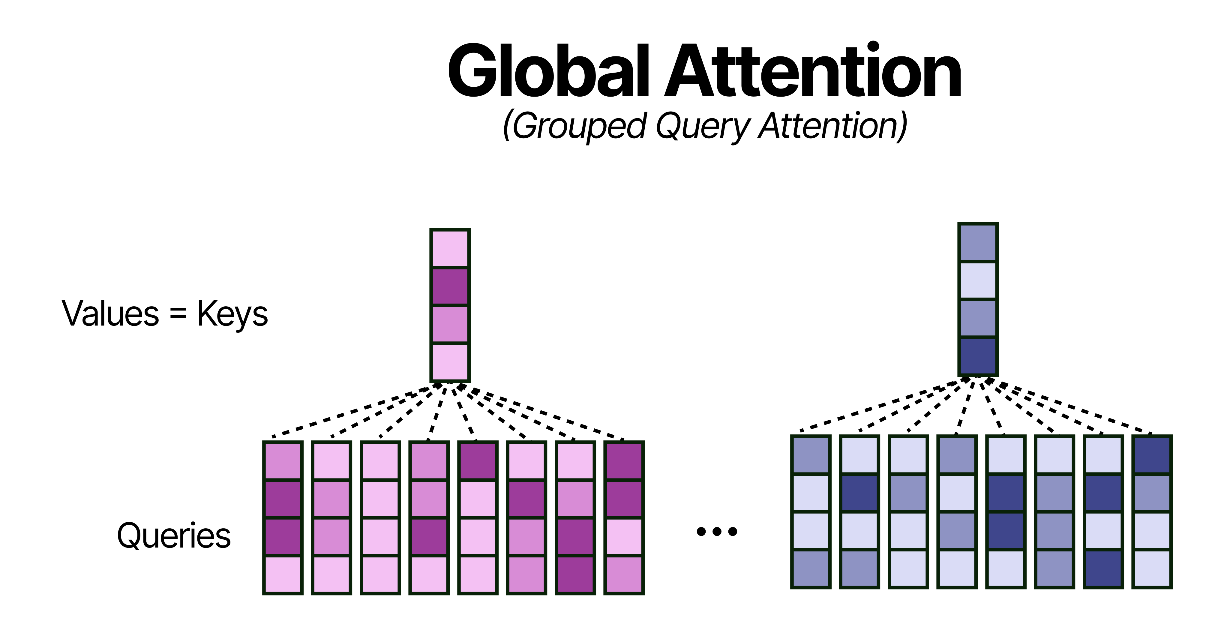
K=V
Despite the improvements to the grouping in Grouped Query Attention, the global attention layers still take up quite a bit of memory since they attend to the entire sequence. Grouping into 8 queries helps a bit but there is more that can be done for efficiency! (View Highlight)
A neat trick, that does not hurt performance that much, is by using the Keys and Values only in the global attention layers. Effectively, this means that all Keys are equivalent to the Values which further reduces the memory requirements for the KV-Cache (or perhaps more accurately now the K-cache for the global attention layer).
(View Highlight)
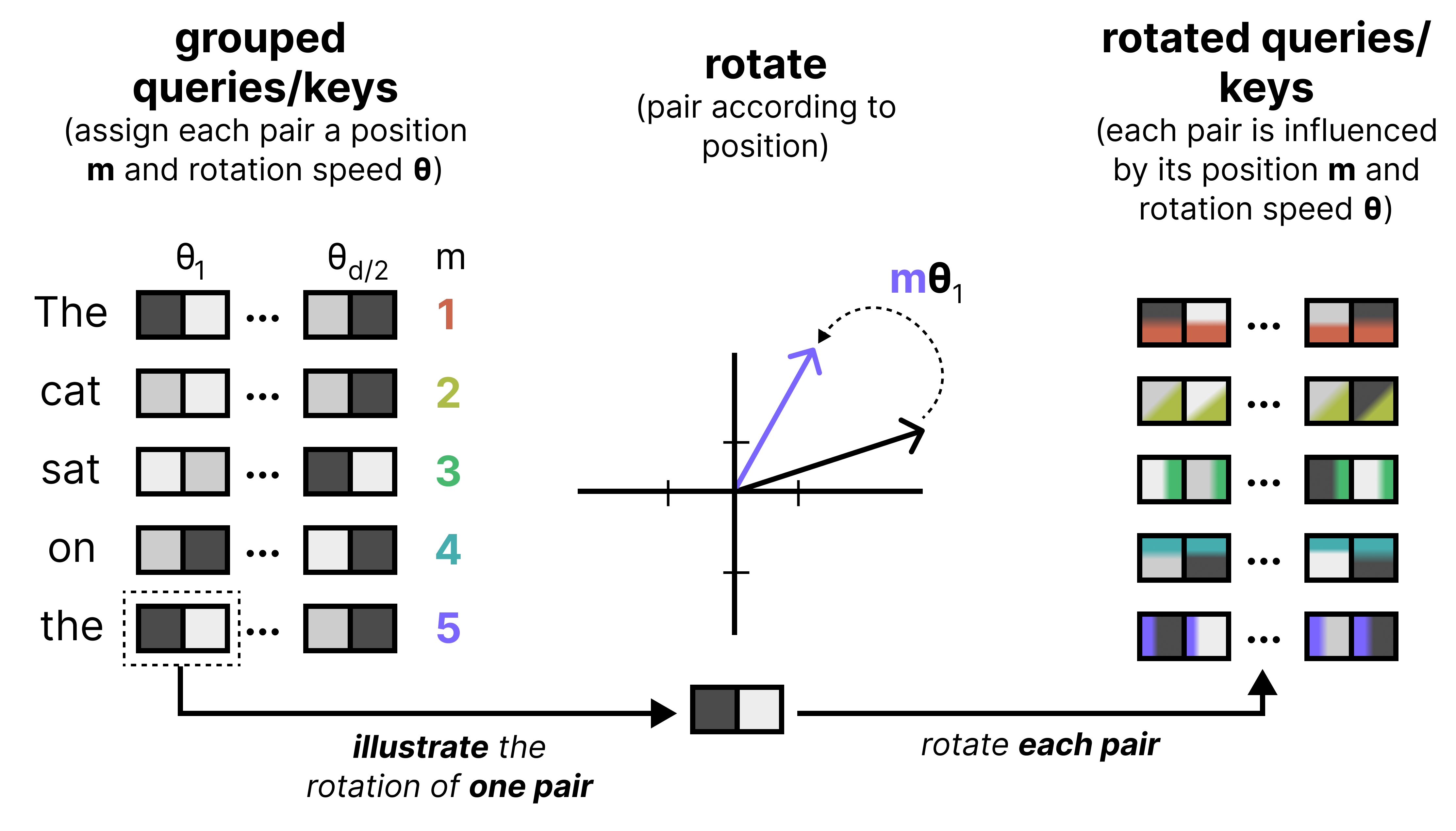
An important component of any Large Language Model is how it keeps track of the order of words in a sequence. One of the most common techniques is called Rotary Positional Encodings (RoPE). RoPE takes the Query and Key vectors and slices them up into pairs of two values. Each pair can now be seen as a vector in 2-dimensional space pointing towards a direction. RoPE rotates this direction slightly for each pair of values at decreasing speeds. The first pair has a large rotation compared to the last pair. This rotation allows the model to track the relative distances between words.
(View Highlight)
 (View Highlight)
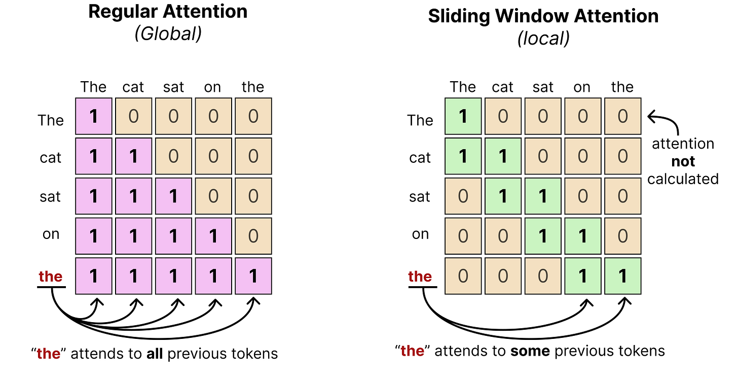 (View Highlight)
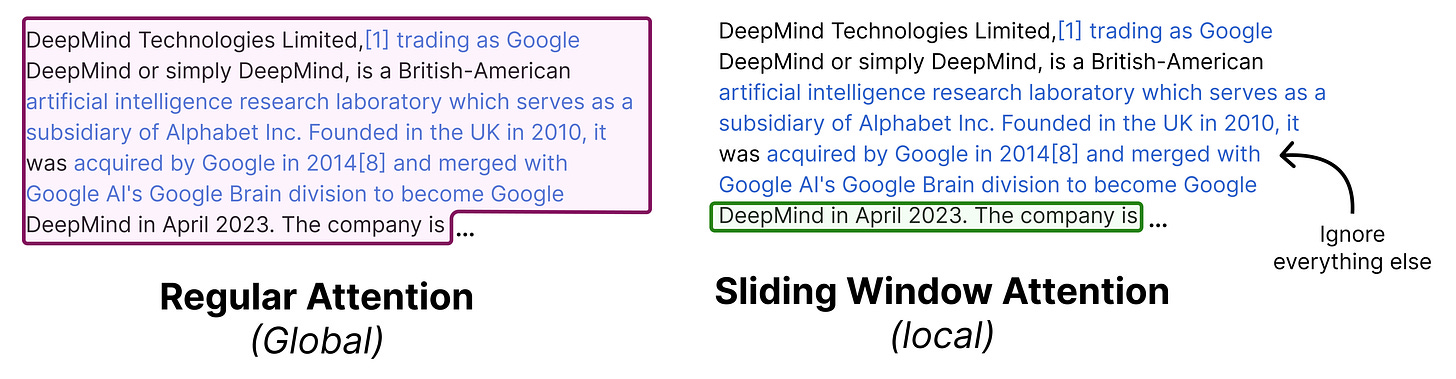 You typically fix the number of tokens it can see previously. In the case of Gemma 4 models, the smaller models (E2B and E4B) have a sliding window of 512 tokens and the larger models (26B A4B and 31B) have a sliding window of 1024 tokens. (View Highlight)
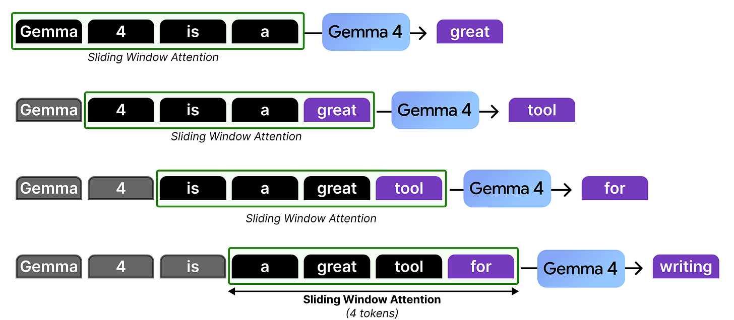 In our example, there is only attention given to the last four tokens which at some point in the generation starts to “ignore” the ones that came before that. However, it is actually not forgetting the representations that it calculated in the previous steps. The hidden states allow for the attention to be passed along the attention mechanism from previous layers and steps all the way to the current token.
(View Highlight)
In our example, there is only attention given to the last four tokens which at some point in the generation starts to “ignore” the ones that came before that. However, it is actually not forgetting the representations that it calculated in the previous steps. The hidden states allow for the attention to be passed along the attention mechanism from previous layers and steps all the way to the current token.
(View Highlight) Although information can be propagated by stacking sliding windows, it is not a perfect recall or attention mechanism. Think of it like a game of telephone, information gets diluted each time it passes through another layer!
Therefore, much like in Gemma 3, local attention and global attention layers are interleaved such that the model does attend to the full sequence at times to better capture the global structure. (View Highlight)
Although information can be propagated by stacking sliding windows, it is not a perfect recall or attention mechanism. Think of it like a game of telephone, information gets diluted each time it passes through another layer!
Therefore, much like in Gemma 3, local attention and global attention layers are interleaved such that the model does attend to the full sequence at times to better capture the global structure. (View Highlight)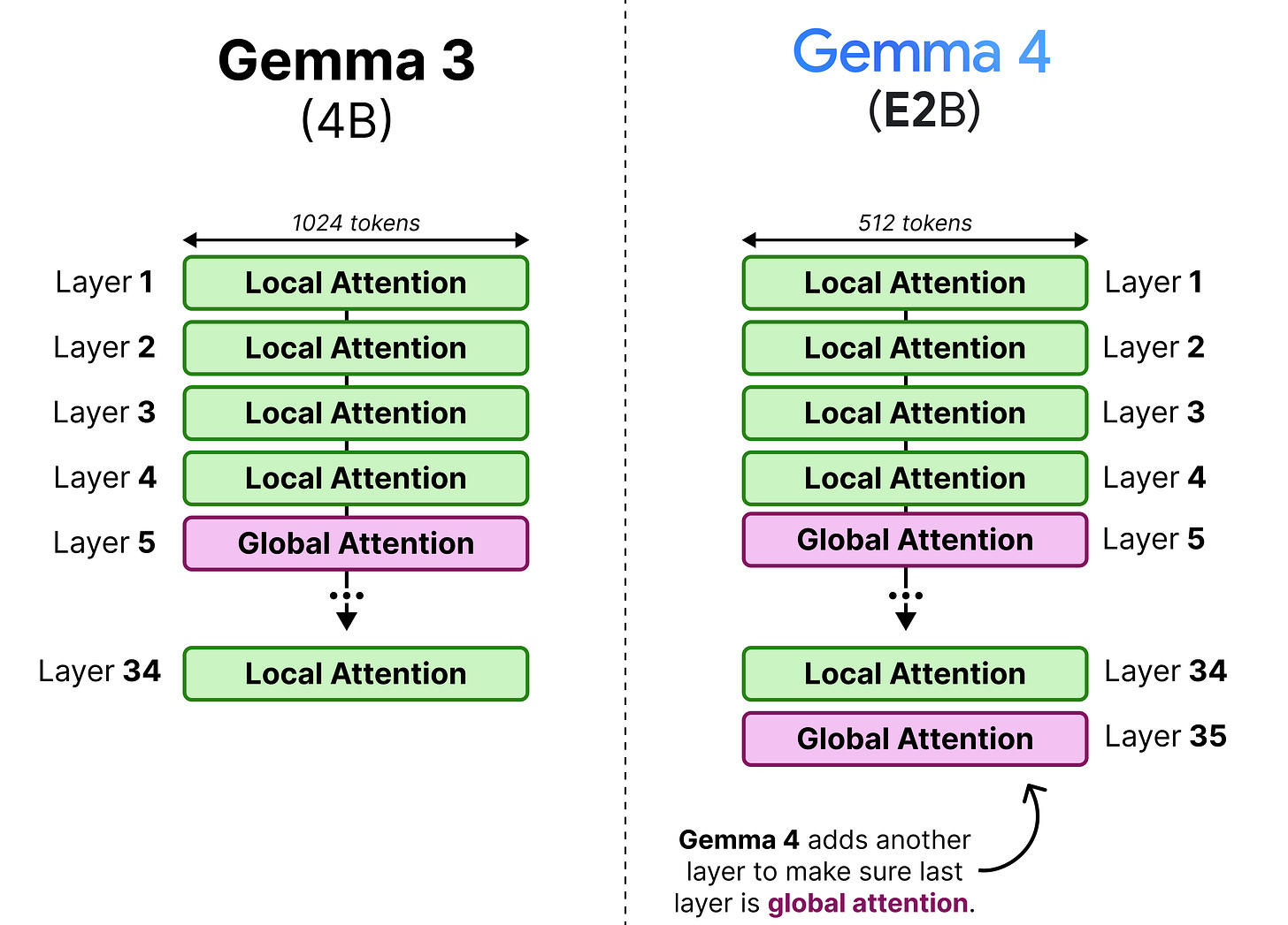 (View Highlight)
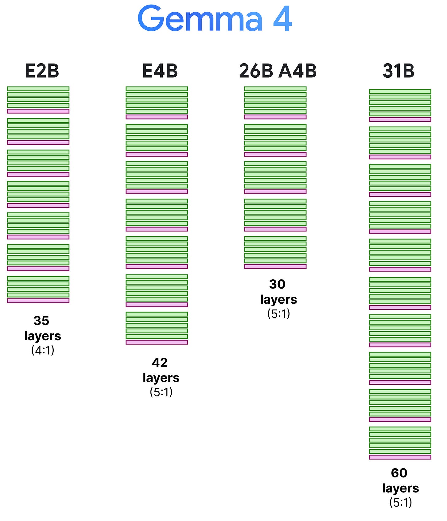 (View Highlight)
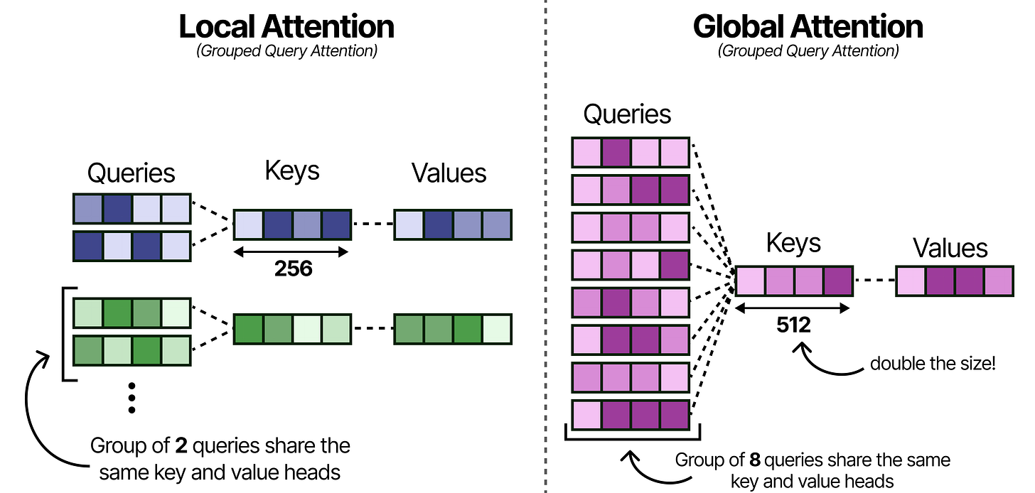 (View Highlight)
 (View Highlight)
 (View Highlight)